My first paper is on arXiv: End-to-end Offline Reinforcement Learning for Glycemia Control. I’m the first author, with Alice Adenis, Erik Huneker and Maxime Louis, from our work at Diabeloop. This post walks through what we did and why, without the full formality of the paper.
Background: closing the loop
In type 1 diabetes, the pancreas no longer produces insulin, the hormone that lets cells take up blood sugar. Patients have to inject it themselves: large boluses at meals, plus a steady basal stream to cover the glucose the body produces on its own. Get the dose wrong and glycemia drifts too high (hyperglycemia, long-term damage) or too low (hypoglycemia, an immediate danger).
A closed-loop system, or artificial pancreas, automates this. A continuous glucose monitor (CGM) reports glycemia every 5 minutes, and an algorithm decides how much insulin the pump delivers. The goal is to keep glycemia in the 70–180 mg/dL range as much as possible.
Why not just use a simulator?
Control algorithms for artificial pancreases are designed and validated almost entirely on virtual patients, because testing on real people is slow, expensive and risky. For simple, conservative controllers (a PID loop, a meal bolus calculator, insulin cut-off when hypoglycemia approaches) that works well: they have high bias, low variance, and are fairly robust to simulator errors.
A reinforcement learning agent trained online on a simulator is a different story. It optimizes against the simulator as hard as it can, and it will exploit any of its biases. Known examples include simulated patients whose glycemia never plateaus after a meal, or hypoglycemia dynamics that don’t match real data. An agent that has learned these quirks can behave badly on a real patient, which is not acceptable for a device that doses insulin.
Offline RL removes the simulator from training. The agent learns only from data logged by an existing policy, with no exploration. That fits this setting well:
- closed-loop systems already in use generate a lot of real data;
- existing controllers are safe and validated by diabetologists, so a good new policy should stay reasonably close to them, which is exactly what offline RL algorithms enforce.
Framing glycemia control as RL
Data. We used real-life data from the DBLG1 closed loop, which equips more than 10,000 patients. We randomly picked 100 patients who had agreed to share their data, and kept only days where the closed loop was active more than 70 % of the time: 6.9 million transitions in total, with patients observed for about 284 days on average. The behavior policy isn’t exactly the DBLG1 algorithm: patients sometimes modify or add boluses, and adjust some parameters. We see this as a benefit, because it widens the range of actions in the data.
State. After testing several combinations, the best state was: the last hour of glycemia and insulin delivery, insulin on board (IOB, insulin injected but not yet active), carbohydrates on board (COB, undigested carbs from declared meals), total daily dose (a proxy for the patient’s insulin needs) and the time of day (insulin sensitivity follows a circadian rhythm).
Action. A basal insulin rate between 0 and 10 U/h. Meal boluses (1 to more than 15 U) are by far the largest doses, so we left them to a standard, deliberately cautious meal bolus calculator. The agent can still add insulin after a meal, but it can never prescribe a large dose on its own. On top of that, a safety rule stops all insulin when a linear regression on recent glycemia predicts hypoglycemia within the next 15 minutes to 1 hour.
Horizon. With 5-minute steps and $\gamma = 0.99$, the effective horizon is $1/(1-\gamma) \approx 100$ steps, about 8 hours. That matches how long a meal or a bolus keeps affecting glycemia.
Reward. Glycemia control has no natural reward, and the reward decides everything the agent learns. We kept rewards that depend only on the current glycemia and compared four candidates:
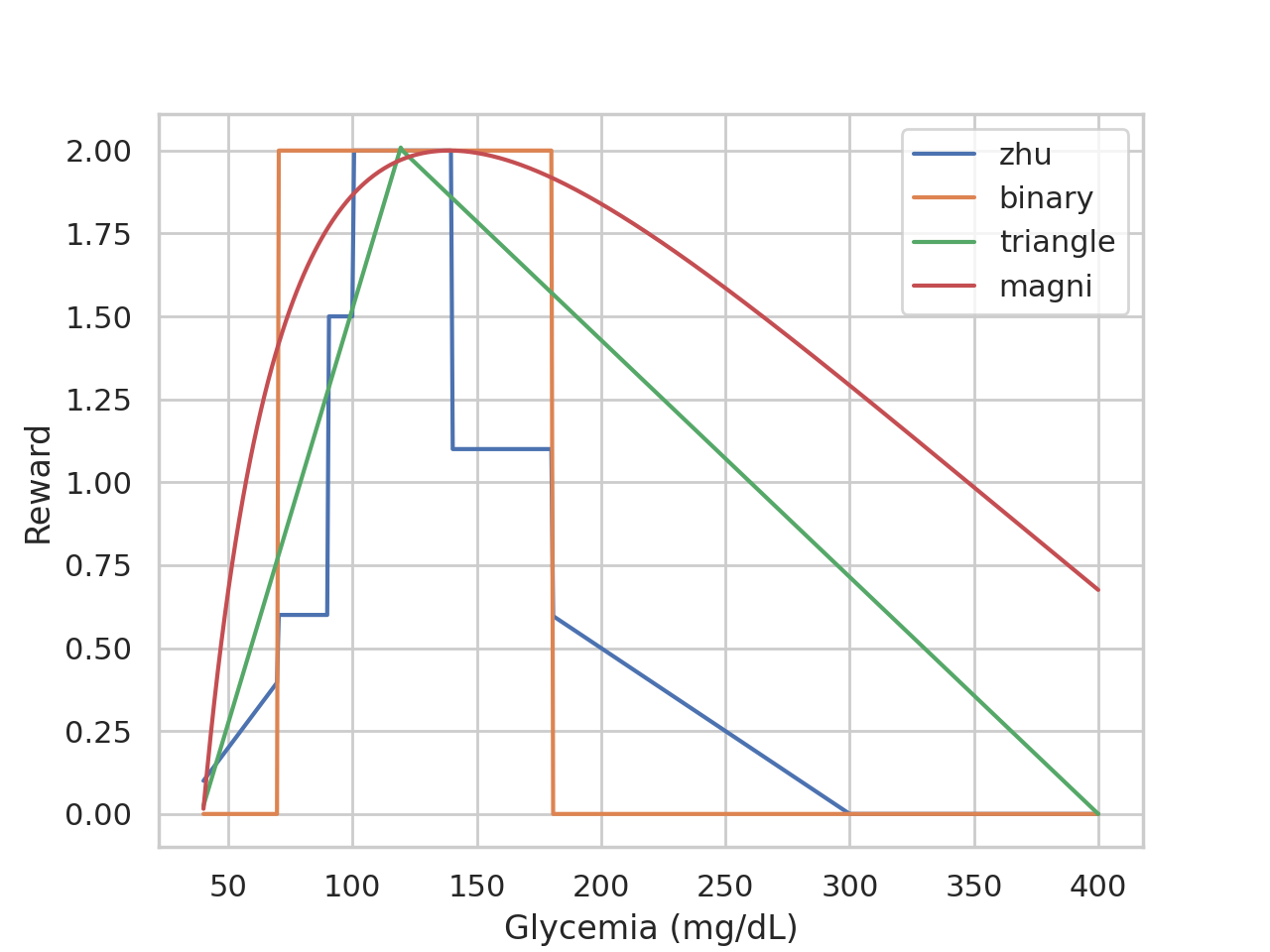
Candidate reward functions as a function of glycemia. Each makes a different trade-off between hypo- and hyperglycemia.
To choose without training an agent per reward, we checked, for each patient-day, how well the total reward correlated with the clinical metrics. Magni and triangle correlated least with time in range and time below range. The binary reward, which is just time in range, carries no signal once glycemia is above 180 mg/dL, so agents trained on it sometimes failed to bring glycemia down after meals. The stepwise reward from Zhu et al. is the one used for the results below.
Three offline RL algorithms
The core difficulty of offline RL is distribution shift: as soon as the new policy acts differently from the behavior policy, it reaches states and actions the data doesn’t cover, and Q-value estimates there can be wildly optimistic. Each algorithm we compared handles this differently:
- BCQ (Batch-Constrained Q-learning) uses a variational autoencoder to propose only actions that look like those in the data, then picks the one with the highest Q-value.
- CQL (Conservative Q-learning) learns a lower bound on the Q-function, pushing down the values of out-of-distribution actions.
- TD3-BC adds a behavior cloning term to the TD3 actor loss, so the policy maximizes Q while staying close to the logged actions.
We tuned state composition, reward and key hyperparameters (such as TD3-BC’s RL/BC trade-off) iteratively, A/B-testing style, on a limited compute budget.
Results of the population model
We evaluated the agents on a simulator. That may sound contradictory, but here the simulator is only a sanity check: passing it is necessary, not sufficient. TD3-BC came out best and improved on the behavior policy for every metric except the coefficient of variation, which stayed within clinical targets:
| Time in range (70–180) | Below 70 | Below 54 | Above 180 | Mean glycemia | |
|---|---|---|---|---|---|
| Behavior policy | 69.9 % | 3.6 % | 1.4 % | 26.5 % | 156.6 mg/dL |
| BCQ | 70.4 % | 3.9 % | 1.0 % | 25.7 % | 147.9 mg/dL |
| CQL | 57.8 % | 9.9 % | 5.1 % | 32.3 % | 150.8 mg/dL |
| TD3-BC | 74.4 % | 2.7 % | 0.9 % | 22.9 % | 148.6 mg/dL |
Looking at a simulated day shows how the agent differs:
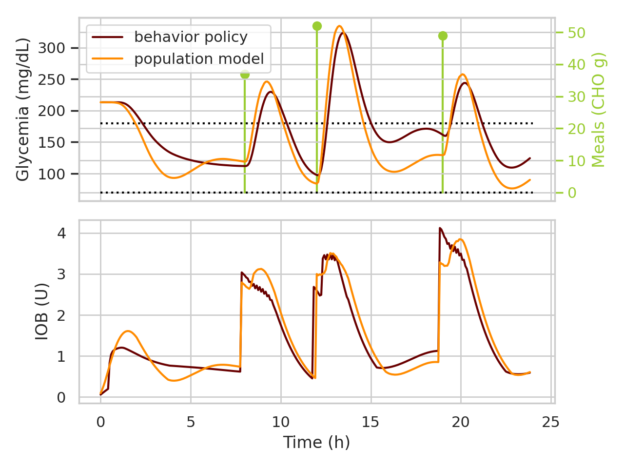
One simulated day. Top: glycemia, with meals in green. Bottom: insulin on board. The RL agent brings glycemia down faster at the start, and adds more insulin about an hour after each meal.
The agent is more aggressive when glycemia is high, but it also eases off earlier when glycemia is high and already falling. Around meals, it adds noticeably more insulin about an hour after the bolus.
We also tested the harder case of unannounced meals: no meal bolus and no carbohydrate information, so the agent has to react to glycemia alone. Compared with the behavior policy, the RL agent raised time in range by 8.0 %, cut time below range by 6.1 % and lowered mean glycemia by 13.2 mg/dL. It’s an early step towards a loop that doesn’t need patients to declare their meals.
Personalization without a simulator
Current closed loops vary a lot from one patient to the next: in our simulations, time in range ranged from about 50 % to over 80 %. The natural next step is to fine-tune the population agent on each patient’s own data. But how do you check that a personalized agent is better, if you don’t trust a simulator and can’t test on the patient?
Estimating clinical metrics with FQE
Fitted Q evaluation (FQE) estimates the value of a new policy $\pi$ from logged transitions $(s_t, a_t, s_{t+1})$ by fitting the Bellman equation
$$ Q(s_t, a_t) = c(s_t, a_t) + \gamma\, Q\big(s_{t+1}, \pi(s_{t+1})\big) $$The key observation is that the cost $c$ doesn’t have to be the reward the agent was trained on. Choose the indicator of normal glycemia, $c_{\text{TIR}}(x) = \mathbf{1}[70 \le x \le 180]$. Its expected value under $\pi$ is the fraction of time spent in range, so the learned Q-value becomes
$$ Q(s, a) = \mathbb{E}\left[\sum_{k=0}^{\infty} \gamma^k c_{\text{TIR}}(s_k)\right] = \frac{\text{TIR}^\pi}{1-\gamma} $$Swapping in $\mathbf{1}[x < 70]$ or $\mathbf{1}[x > 180]$ gives time below and above range. Instead of a hard-to-interpret Q-value, FQE now reports the metrics diabetologists actually use, for a policy that has never been run on anyone. One caveat: FQE estimates are known to be better at ranking policies than at giving exact values.
The protocol
Each patient’s history is split chronologically into four equal parts:
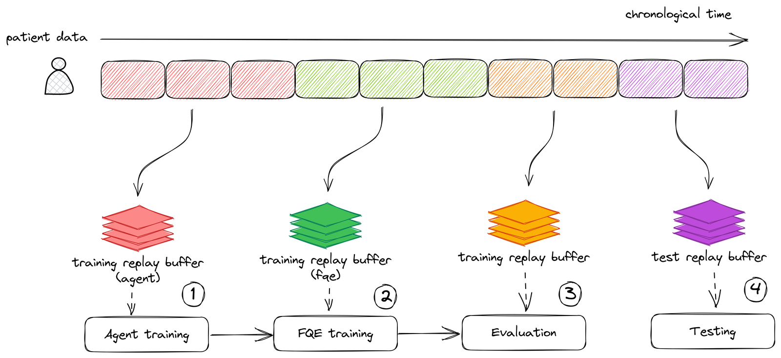
Personalization protocol: fine-tune the agent, train FQE models, select the best checkpoint, then measure on held-out data.
- fine-tune the population agent on the first quarter;
- train one FQE model per metric (reward, time in range, below, above) on the second;
- use the third to pick the best checkpoint, guarding against overfitting and catastrophic forgetting;
- report final estimates on the last quarter, which was never used before.
The population model gets FQE models trained on the same data, so both are compared on equal footing. For these experiments we turned off the meal bolus calculator and the hypoglycemia cut-off, to measure the agent on its own.
What personalization changes
We ran this on 25 new patients, not in the training set, each observed for about 333 days, so about three months of data went into fine-tuning.
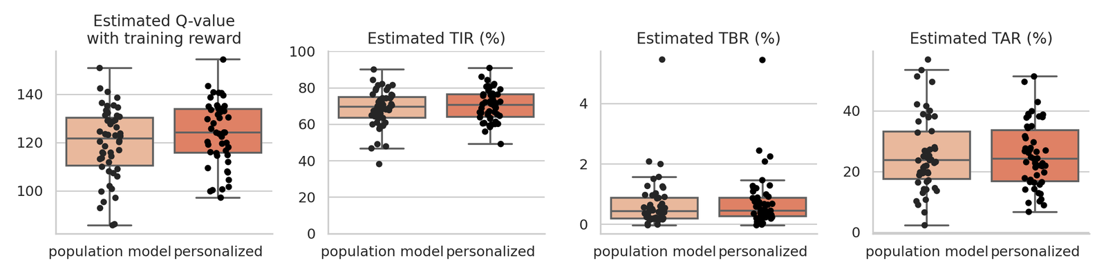
FQE estimates before and after personalization, one dot per patient.
On average, the estimated training reward went up and time in range improved by about one point, while time below and above range stayed essentially flat. The clearest gain is for the patients who needed it most: the lowest estimated time in range went from 38 % to 50 %.
To check that the agents learned something sensible, we used a simple fact: insulin has its largest effect about 30 minutes after delivery. So if glycemia was high 30 minutes later in the real data, a better controller should have delivered more insulin, and less if it was low.
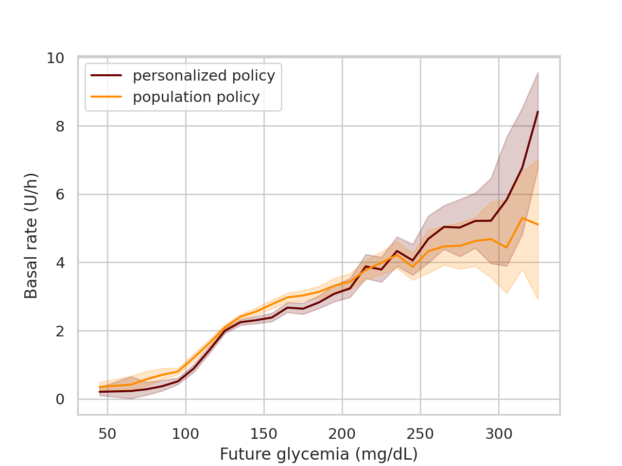
Basal rate chosen by each policy as a function of the glycemia 30 minutes later. Personalized agents deliver less insulin below 200 mg/dL and more above.
That is what happens: personalized agents send less insulin when glycemia is heading below 200 mg/dL and more when it is heading above.
Limitations and next steps
- The population results come from simulation; the personalization results are FQE estimates. Neither replaces a clinical evaluation.
- FQE is better at ranking policies than at exact values, and how its accuracy depends on the data distribution deserves a proper study.
- An ablation removing manually modified boluses from the data would show whether they really help offline training.
Read more
- Paper: arXiv:2310.10312
- Code: offline RL agents on GitHub
All figures are from the paper.
Citation
@misc{beolet2023endtoend,
  title         = {End-to-end Offline Reinforcement Learning for Glycemia Control},
  author        = {Beolet, Tristan and Adenis, Alice and Huneker, Erik and Louis, Maxime},
  year          = {2023},
  eprint        = {2310.10312},
  archivePrefix = {arXiv},
  primaryClass  = {cs.AI}
}